CCE 102 Grade Analysis – Greg Macfarlane

I taught four sections of CCE 102 this year. This post serves to document and record how the students performed in each section and by major. Across the four sections, 238 students completed the course. The average GPA by section has not been consistent across all four sections, however.

data |>
  group_by(semester, section) |>
  summarise(count = n(), `gpa` = mean(final_gpa)) |>
  kbl(digits = 2, col.names = (c("Semester", "Section", "Count", "Average GPA"))) |> 
  kable_styling()

`summarise()` has grouped output by 'semester'. You can override using the
`.groups` argument.

Semester	Section	Count	Average GPA
Fall 2024	001	60	3.52
Fall 2024	003	53	2.95
Winter 2025	001	60	3.03
Winter 2025	003	65	3.24

As a note, I am only including the courses where I was the primary instructor. Darrell Sonntag taught an additional section each semester, but he and I had slightly different assignments and grading policies to the point where I don’t think it would be productive to compare them.

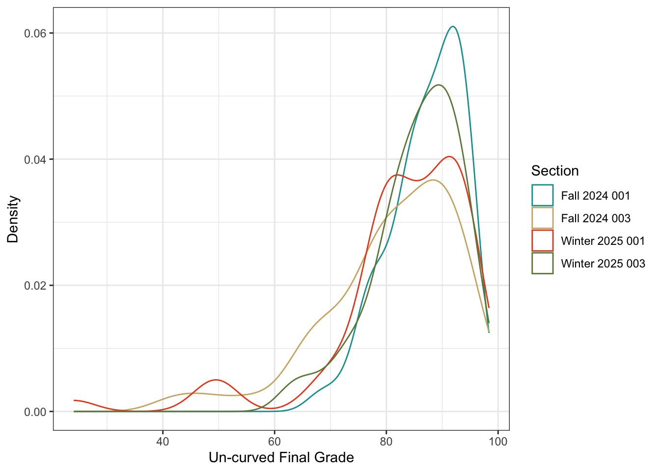
Let’s look at the distribution of grades by section (see Figure 1). These percentile grades do not include any final curve adjustments. Each section reached its GPA in different ways. Fall 2024 section 003 had a number of students earning low but passing C grades, while Winter 2025 001 had a few students perform poorly and earn E grades.

ggplot(data, aes(x = current_pct, color = str_c(semester, section, sep = " "))) + 
  geom_density(alpha = 0.25) +
  scale_color_manual("Section", values = pal) +
  theme_bw() + xlab("Un-curved Final Grade") + ylab("Density")

Figure 1: Grade distribution by section.

Winter 2025 felt much better in terms of student attitude and workload. At the same time, the average grades were a little bit lower. I’m curious how the student evaluations shake out.

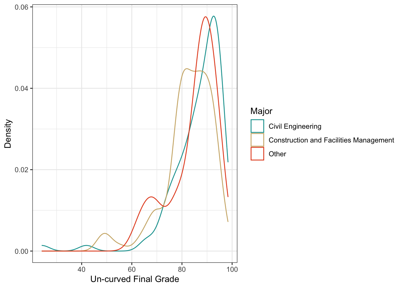
Now let’s consider the breakdown across majors, which I show in Figure 2. Note that this is a GE class, with 10 different majors enrolled. However, 92% of students are enrolled in either Civil Engineering (CE) or in Construction and Facilities Management (CFM), where this class is required. CE students do better in the class, with the mode being about an A-. CFM majors have a wide distribution, but the mode is in the B range. Other majors — including a few environmental science students and multiple open majors — perform more like CE students, with a few poor performing exceptions.

ggplot(data, aes(x = current_pct, color = major)) + 
  geom_density(alpha = 0.25) +
  scale_color_manual("Major", values = pal) +
  theme_bw() + xlab("Un-curved Final Grade") + ylab("Density")

Figure 2: Grade distribution by section.

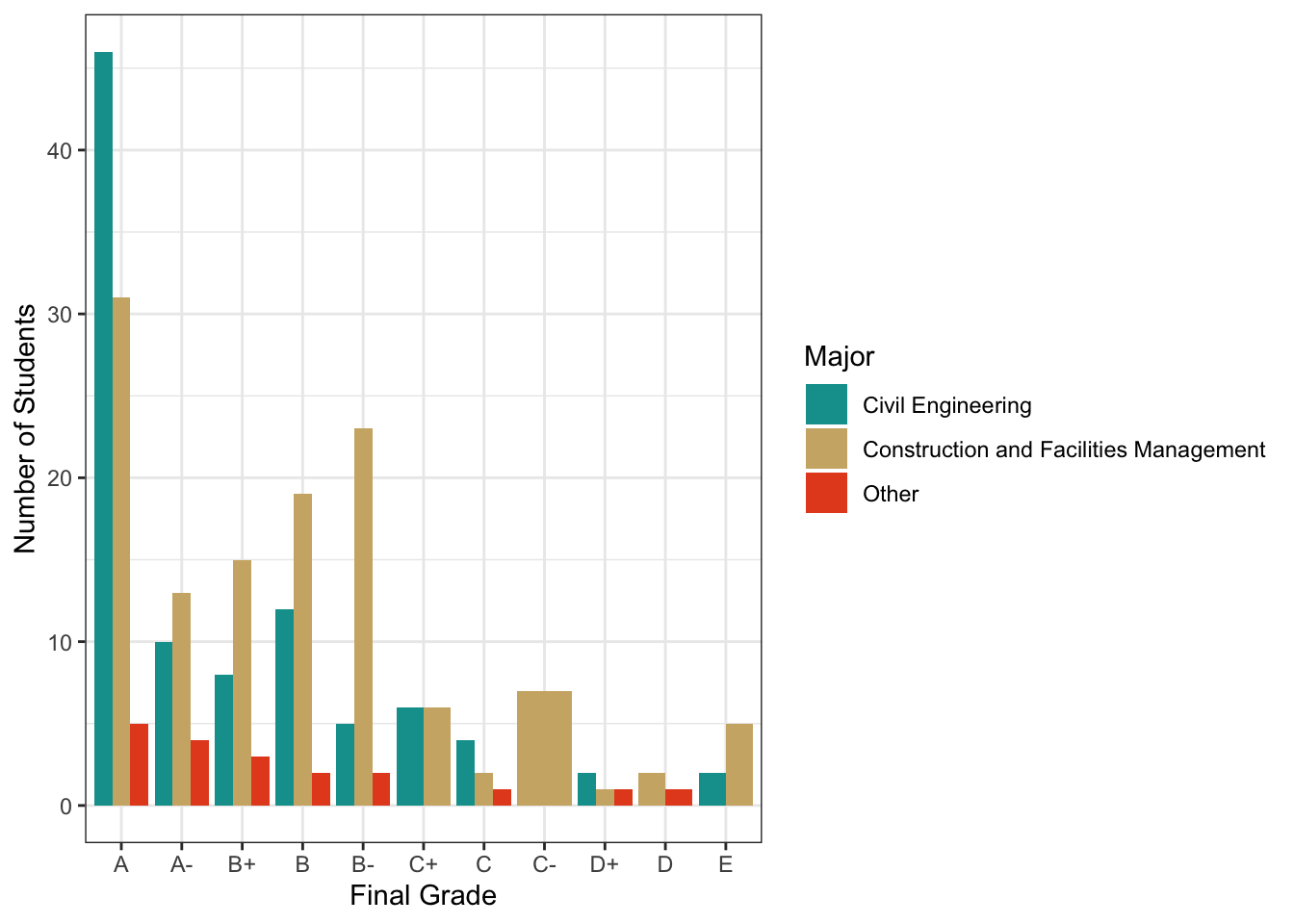
The final grades awarded by all semesters (including with a curve applied) are shown in Figure 3. The most common grade awarded to all students in all majors is an A, particularly when combined with the A- grades. But there are probably too many CFM students earning B- and C grades to make me happy.

data |>
    mutate(final_grd = factor(final_grd, levels = c("A+", "A", "A-", "B+", "B", "B-", "C+", "C", "C-", "D+", "D", "D-", "E", "W"))) |>
    ggplot(aes(x = final_grd, fill = major)) +
    geom_bar(, position = "dodge") +
    xlab("Final Grade") + ylab("Number of Students") +
    scale_fill_manual("Major", values = pal) +
    theme_bw()

Figure 3: Final Grades awarded by major, all semesters.

The chart above does not contain withdrawals, as students who withdraw do not remain on my rolls. I cannot therefore track what major the withdrawn students are enrolled in. But I can compute the overall DEW rate for both semesters, shown in Table 1. This rate has come down, but it would be nice to get it below 5%.

# withdrawals
withdrawals <- tibble(semester = c("Winter 2025", "Fall 2024"), w = c(3, 4))

data |>
    mutate(de = case_when(
      str_detect(final_grd, "D") ~ TRUE,
      str_detect(final_grd, "E") ~ TRUE,
      TRUE ~ FALSE
    )) |>
    group_by(semester) |>
    summarise(n = n(), de = sum(de))  |>
    left_join(withdrawals, by = "semester") |>
    mutate(dew = (de + w) / (n + w) * 100)  |>
    kbl(col.names = c("Semester", "N Complete", "D/E", "W", "DEW [%]"), digits = 2)  |>
    kable_styling()

Table 1: DEW Rate by Semester

Semester	N Complete	D/E	W	DEW [%]
Fall 2024	113	7	4	9.40
Winter 2025	125	7	3	7.81